>

Forced Oscillations

Section 3.8 in Greenberg

10/2/2000

Richard Hitt

Introduction

State the purpose of the worksheet.

Getting started

Every Maple worksheet should begin by re-initializing the Maple "kernel" and loading the additional packages that we are most likely to use.

> restart;

> with( plots ):

> with( DEtools ):

Warning, the name changecoords has been redefined

Undamped Case

In this worksheet we examine the solution to an initial value problem with periodic forcing function with different forcing frequencies. Of particular interest is the behavior of the solution as the forcing frequency approaches the natural frequency of the equation, i.e. , when resonance occurs..

> MODEL := diff( y(t), t$2 ) + 2 * y(t) = 3*sin( omega*t );

> IC := y(0)=1, D(y)(0)=0;

> VAR := { y(t) };

>

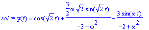
> sol1:=dsolve( { MODEL, IC }, VAR );

Note that this solution contains two terms which appear in the homogeneous solution and one term that is a particular solution to the nonhomogeneous equation.

>

The natural frequency is . The following plots provides an animated view of the solutions as increases towards .

> Omega := [ 0,0.1,0.2,0.3,0.4,0.5,0.6,0.7,0.8,0.9,1.0,1.1,1.2,1.25,1.3,1.35, 1.4 ]:

> P := seq( plot( eval( rhs(sol1), omega=w ), t=0..100 ), w=Omega ):

> display( P, insequence=true );

What do you notice about the amplitude of the solutions? What would happen if ?

>

> sol2:=dsolve( eval( { MODEL, IC }, omega=sqrt(2) ), VAR );

Notice that this solution is significantly different from the general solution when is not . The particular solution has an amplitude that grows linearly with time - this is RESONANCE.

> plot(rhs(sol2),t=0..50);

>

Damped Case