>

MA 507

Chapter 5: Laplace Transforms

16 October 2000

Richard Hitt

Introduction

This worksheet gives a few of the basics on using Maple with Laplace transforms.

Getting Started

We have to load the integral transforms package if we want to use the built-in Maple function for the Laplace transform and its inverse.

> restart;

> with(inttrans);

>

The Basics

Recall the definition of the Laplace transform:

.

We can use Maple to calculate the Laplace transforms of functions. The syntax is illustrated below where we let Maple calculate the transform of .

> laplace(t,t,s);

Of course, Maple can calculate transforms of many functions.

> laplace(sin(t)*exp(t),t,s);

> laplace(BesselJ(0,t),t,s);

> laplace(diff(y(t),t)+2*y(t)=sin(t),t,s);

Maple can compute inverse Laplace transforms as well.

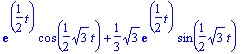
> invlaplace(s/(s^2-s+1),s,t);

Solving an IVP with Laplace Transforms

Maple can be used to solve differential equations via Laplace transforms. For the first example, we use Maple to perform each step along the way.

Example 1

> de1 := diff(y(t),t)+2*y(t)=sin(t);

We can use laplace( , , ) to transform the entire DE.

> lode1:=laplace(de1,t,s);

We can also impose an initial condition like .

> livp1:=subs(y(0)=1,lode1);

If we let denote the laplace transform of , the above equation is . In order to solve the equation for , we can use

> Y1 :=solve(livp1,laplace(y(t),t,s));

We can find the solution to the original IVP by taking the inverse Laplace transform of :

> invlaplace(Y1,s,t);

Maple can automate the entire process using the method=laplace option in dsolve.

> dsolve({de1,y(0)=1},y(t), method=laplace);

Note: You will get the same result in this case if you don't specify "method=laplace" in the dsolve command. This is not always the case, though.

>

Other Examples

Example 2

> ode1:=diff(y(t),t$2)+y(t)=Heaviside[t-Pi]*cos(t);

> ic1:=y(0)=0,D(y)(0)=0;

> soln1:=rhs(dsolve({ode1,ic1},y(t),method=laplace));

> plot(soln1,t=0..30);

>

Example 3

> ode2:=diff(y(t),t$2)+0*diff(y(t),t)+4*y(t)=2*Heaviside[t-Pi]-Heaviside(t-2*Pi);

> ic2:=y(0)=1,D(y)(0)=0;

> soln2:=rhs(dsolve({ode2,ic2},y(t),method=laplace));

> plot(soln2,t=0..15);

>

Square Waves

We define a square wave function in Maple as follows

> sqw := proc(t,d,T) piecewise(t-floor(t/T)*T<(d/100)*T, 1) end;

so that sqw[t,d,T] gives a function having value 1 d% of the time with period T. For example,

> plot(sqw(t,50,4),t=0..10);

> dsolve({diff(y(t),t$2) + 2*diff(y(t),t) + 4*y(t) = sqw(t,50,4), y(0)=1, D(y)(0)=2},y(t),method=laplace);

But Maple is not able to handle the integration directly. So we can define a square wave over a finite interval using sums of Heaviside functions. For example

> E := sum(Heaviside(t-2*k)-Heaviside(t-2*k-1),k=0..10);

> plot(E,t=0..30);

Then Maple can solve a DE built with such a finite square wave.

> ode3:=diff(y(t),t$2) +0*diff(y(t),t) + 4*y(t) = E;

> sol3:=dsolve({ode3, y(0)=1, D(y)(0)=1},y(t), method=laplace);

> plot(rhs(sol3),t=0..20);

>

An RLC Circuit

We wish to analyze a series RLC circuit having an applied voltage which is a square wave. Specifically, we would like to find the initial conditions which completely eliminate any transient in the circuit. The relevant differential equation is 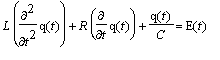with initial conditions and where q = q(t) is the charge on the capacitor. We will assume L=1 henry, R = 3 ohms, C = 1/2 farad, and is a square wave function starting with value 1 and alternating from 1 to 0 to 1 across each unit interval.

Exercise: By trial and error, find a set of initial conditions that give a periodic solution, i.e., that produce no transient.

Dirac Delta

For convenience, we define a shorthand name for the Heaviside function:

> H := t -> Heaviside(t);

This pulse function corresponds to what we will refer to as in class if we use :

> pulse := (t,h) -> (1/h)*H(t)*H(h-t);

Let's graph the pulse for several values of h:

> plot( [pulse(t,1),pulse(t,1/2),pulse(t,1/4),pulse(t,1/5),pulse(t,1/6)], t=-0.5..1.5, color=[red,blue,green,black,brown], title=`Pulse functions for h = 1, 1/2, 1/4, 1/5, 1/6`);

Maple can compute the Laplace transforms of Dirac delta functions.

> laplace(Dirac(t),t,s);

> laplace(Dirac(t-2),t,s);

Here is an example.

> ode10:= diff(y(t),t$2)+2*diff(y(t),t)+4*y(t)=Dirac(t-1);

> sol10:=dsolve([ode10,y(0)=0,D(y)(0)=0],y(t));

> plot(rhs(sol10),t=0..10);

>

Additional Exercises

In addition to the exercise in the RLC circuit section, work the following.

Exercises 6(g,j), 7(g,j) on page 275, and 1(c,f) on page 280. Graph all the solutions.